Breaking Algorithms - SMT Solvers for WebApp Security
*
Introduction
This post introduces Z3; an MIT licensed SMT solver from Microsoft Research. We’ll discuss some typical uses of SMT solvers, show how to generate constraints using Z3’s Python bindings and provide an example for the use of this technology for WebApp security.
SMT solvers find use in a wide range of fields. The approach was applied to everything from predicting genomic regulatory logic (see The Varied Forms of Verification with Z3 by Microsoft Research for an overview of Z3 applications) to designing microfluidic systems and validating cloud network configurations. Essentially, SMT solvers provide a formal approach to exploring and reasoning about complex, inter-dependent systems.
One important application of SMT solvers is formal verification, e.g., symbolic execution of software, input analysis, and security testing. Some actively-maintained tools in this category include SAGE from Microsoft Research, KLEE, S2E, and Triton. SMT solvers that are particularly useful for symbolic-execution applications include Z3, STP, Z3str2, and Boolector.
This post is structured as a set of three tutorials. The first part contains an introduction to Z3’s Python bindings and demonstrates how to generate constraints and solve them. The second part introduces the concept of a Linear Congruential Generator and demonstrates how Z3 can be used to predict PRNG output. Finally, the third part extends the model used in the second section to demonstrate real-world use of the approach using OWASP Benchmark.
Note on running these examples: Z3 is non-trivial to install. As such, we recommend using the Dockerfile available here to set up Z3 with Jupyter notebook and all required dependencies.
Table of Contents
- Introduction
- Part 1 - Introducing Z3
- Part 2 - Modeling a PRNG Algorithm
- Part 3 - Extending our approach to a real-world example
- Final words
- Notes & Sources
- Background
Part 1 - Introducing Z3
Before we delve into more complex problems, we’ll demonstrate how to model a mathematical puzzle. During this section, we’ll be somewhat verbose in describing the logic and execution flow. We aim to familiarize the reader with developing constraints using Z3’s Python bindings. As such, feel free to skip to part 2 if you’re familiar with Z3.
As our toy problem, we’ll use a typical programming puzzle: write a function that accepts two parameters N & n and returns a boolean. The function checks if there are n consecutive, natural numbers (excluding zero) so that \(\sum_{i=1}^n a_i = N\).
If you remember your arithmetic progressions, the sum can be calculated using Gauss’s trick:
\[N = \frac{(a_1 + a_n) \times n}{2}\]Or in our simplified case:
\[N = \frac{(a_1 + (a_1 + 1 \times (n -1))) \times n}{2}\] \[2 \times N = (a_1 + (a_1 + 1 \times (n -1))) \times n\] \[\frac{N}{n} - \frac{n -1}{2} = a_1\]Using this formula, we can calculate a candidate for \(a_1\). If our candidate is a natural number, the function should return true. Otherwise, it should be false. The code for this problem, while simple, requires some derivation (and actually remembering Gauss’s trick).
Now let’s think about this problem as a system of constraints. Obviously, our first constraint is:
\[a_{i+1} = a_i + 1\]Additionally, we should have a constraint for the sum:
\[\sum_{i=1}^n a_i = N\]Let’s translate these constraints into a Z3 model:
import z3 as z
z.set_param('parallel.enable', False)
First, let’s define our goals:
n = 3
N = 1050
Next, we’ll generate some symbolic variables. Symbolic variables (as opposed to concrete variables, which we’ll use later) act as placeholders. They behave like a typing mechanism for Z3 and help it choose suitable solution strategies. Furthermore, as long as the model is satisfiable, symbolic variables can be used to extract concrete values from a model.
Note the use of list comprehension (later we’ll be using dictionary comprehension extensively) and f-strings to generate multiple symbolic variables with unique names.
ints = [z.Int(f'int_{i}') for i in range(n)]
Now we’ll instantiate a solver object. The solver object accepts constraints checks if they are satisfiable. The solver can be tweaked with specific strategies, given intermediate goals, and acts as the front-end to Z3. To solve our problem, we’ll set (in SAT solver lingo, we assert) three constraints:
\(1.\,\,\,\, a_0,\, ...,\, a_{n-1} \in \mathbb{N}\) - non-negative natural numbers
\(2.\,\,\,\, a_{i+1} = a_i + 1\) - consecutive numbers
\(3.\,\,\,\, \sum_{i=1}^n a_i = N\) - sum must equal to some predefined value
s = z.Solver()

for i in range(n-1):
    # Constraint #1
    s.add(ints[i] > 0)
    # Constraint #2
    s.add(ints[i+1] == ints[i] + 1)

# Constraint #3
s.add(z.Sum(ints) == N)
Finally, we’ll use the check() method of our solver object to test the satisfiability of our constraints. The check() method returns one of the following responses: sat, unsat, infeasible, or unknown. Our problem is quite small (in terms of the number of constraints) so we’re only going to get sat/unsat.
if s.check() == z.sat:
    m = s.model()
    print('Found a solution')
    print(f'({n} terms) {m[ints[0]].as_long()} + ... + {m[ints[n -1]].as_long()} == {N}')
else:
    print(f'Finding {n} consecutive integers with a sum of {N} is unsatisfiable')
Found a solution
(3 terms) 349 + ... + 351 == 1050
As can be seen above, the constraints are satisfiable. Notice our use of the model() method to get the model object. We then use our symbolic variables to extract concrete values from the model object using the as_long() method.
Next, we’ll generalize our model and show it can be used to ask a somewhat more complex question.
Notice: our implementation returns the solver object. We consider returning solvers good practice since it allows us to encapsulate constraint construction. The solver can later be used to add additional constraints to describe more complex models.
def build_solver(n: int, N: int):
    # Create symbolic variables
    ints = [z.Int(f'int{i}') for i in range(n)]

    # Instantiate a solver
    s = z.Solver()

    for i in range(n-1):
        # Consecutive numbers
        s.add(ints[i+1] == ints[i] + 1)
        # Non-zero natural numbers
        s.add(ints[i] > 0)

    # Sum
    s.add(z.Sum(ints) == N)

    return s
Using this method, we can seamlessly generate a solver object. Another reason why returning a solver object is good practice is that it lets us inspect our constraints, add additional constraints, force solution strategies, etcetera:
s = build_solver(n = 3, N = 1337)
print(s)
[int1 == int0 + 1,
 int0 > 0,
 int2 == int1 + 1,
 int1 > 0,
 int0 + int1 + int2 == 1337]
Using this approach, we can check if sets of model inputs are satisfiable. For example, below we’re exploring the solution space for N = 1337:
for i in range(3, 10):
    print(f'Sum 1337 is {build_solver(n = i, N = 1337).check()} with {i} integers')
Sum 1337 is unsat with 3 integers
Sum 1337 is unsat with 4 integers
Sum 1337 is unsat with 5 integers
Sum 1337 is unsat with 6 integers
Sum 1337 is sat with 7 integers
Sum 1337 is unsat with 8 integers
Sum 1337 is unsat with 9 integers
Summary: this section introduces Z3 and basic model construction. We demonstrated how to formulate a mathematical problem as a set of constraints, encapsulate the model construction logic into a function and explored the solution space of the problem. In the following section, we’ll demonstrate how Z3 can be used to model an algorithm and using the solver object extract (supposedly) hidden internal states.
Part 2 - Modeling a PRNG Algorithm
After familiarizing ourselves with the basic trappings of Z3, let’s try to apply these skills to a real-world algorithm. During this example we’ll:
- Describe the workings of a popular Pseudo-Random Number Generator (PRNG); the Linear Congruential Generator (LCG)
- Develop a function that symbolically executes an LCG using Z3
- Predict the next value in a sequence of LCG generated numbers
- Extract the value generated before a known sequence of LCG generated numbers
- Extract the seed used to instantiate the PRNG
Linear Congruential Generators (LCGs)
This class of functions generates numbers that have some properties of random numbers (hence pseudo-random). An LCG is a recurrent relation where the initial value (known as a “seed”) goes through mathematical manipulations which produce a new number. The new number becomes the seed used in the next call to the function. This approach is fast, and as long as the parameters (more about them in the next section) are chosen carefully, it can pass some statistical tests for randomness.
For a short intro about LCGs and their limitations take a look at the Wikipedia page about Linear Congruential Generators.
A typical LCG generates a number by performing the following steps:
- Multiply seed by a magic number
- Add another magic number to the result of the multiplication
- Take the modulus of the result with a third magic number
Consequently, the choice of magic numbers for the algorithm is of paramount importance. Poor choice of these parameters can produce strong attractors. Attractors are a feature of dynamical systems where perturbation of the input leads to little or no change in the output (more on attractors can be found here). An example of poor parameter choice can be seen below, where there is a simple multiplication relation between the modulus and the multiplicand. This choice results in strong attractors and short periods (number of calls to the function until a number is repeated):
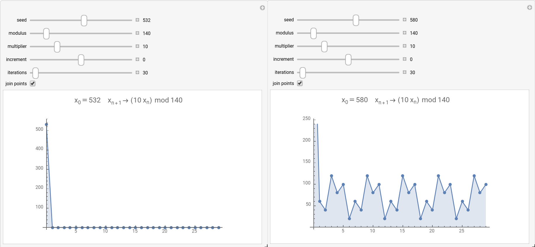
The value on the X-axis in these images represents how many numbers were generated & the Y-axis represents the generated number. For a seed value of 532 (left image), we see the behavior of a strong attractor. Alternatively, for a seed value of 580 (right image), we see an example of short periodicity. Applet used to generate these images is available here.
As can be deduced from the images above, using the magic numbers multiplier=10 & modulus=140 and the seeds 532 or 580, necessarily leads to a strong attractor behavior. Essentially, if these magic numbers are used and one of the two mentioned values gets generated, the rest of the sequence is easily predicable. For example, assuming we chose a seed that is different from 532 and after n calls 532 gets generated, all future numbers in the sequence will be 0. Consequently, even choice of “strong” magic numbers can sometimes lead to poor quality randomness due to the behavior demonstrated above.
As a practical example, we’ll study the LCG implementation in MSVC 2013, which is known to be relatively weak (i.e. poor choice of magic numbers).
Implementation of rand() in MSVC 2013
The algorithm used to implement rand() in MSVC 2013 is a good example of a simple LCG:
static unsigned long int next = 1;

int rand(void)  /* RAND_MAX assumed to be 32767. */
{
    next = next * 214013 + 2531011;
    return (unsigned)(next/65536) % 32768;
}
Based on this snippet, we’d like to generate constraints that simulate the algorithm using Z3. Specifically, we’re interested in the following questions, assuming we have a sequence of numbers generated by the algorithm:
- Can we predict the next value in the sequence?
- Can we calculate the previous number in the sequence?
- What’s the shortest sequence we need to supply Z3 to predict the next number in the sequence correctly?
- Are the solutions unique? Can we find additional internal states that satisfy our constraints?
Now let’s assume we ran rand() 10 times and got the following set of numbers:
4, 54, 63, 79, 13, 55, 76, 11, 14, 45
Let’s construct the constraints required to simulate rand() and answer the above questions. Note: numbers were generated by printing rand() % 100 to constrain the numbers to the [0, 100) range. The seed used to initialize the function was 1337.
Simulating rand() using Z3
In this example, we’ll start using bit vector (BitVec) objects. These objects are symbolic representations of the way data is stored in memory and require a definition of their size. Using bit-vectors allows us to make use of bitwise operators, which we’ll be utilizing extensively in the next example. In this example, we’ll use bit-shifting & the ‘bitwise and’ operators to represent the division and modulus operations.
We’ll start by defining some symbolic variables. We’ll define two variables (output_prev, output_next) to represent the numbers generated before and after the sequence. Besides, we’ll define 10 state_# variables to represent the next variable in the code snippet. Notice the use of dictionary comprehension to generate the state_# variables. Using dictionaries is a useful pattern to hold a large number of symbolic variables in an accessible manner.
output_prev = z.BitVec('output_prev', 32)
states = {f'state_{i}': z.BitVec(f'state_{i}', 32) for i in range(1, 11)}
output_next = z.BitVec('output_next', 32)
Instantiate the solver
s = z.Solver()
Now let’s start adding the problem constraints. Our 1st constraint is that the sequence of numbers was generated by sequential calls to rand(), therefore:
for i in range(2, 11):
    s.add(states[f'state_{i}'] == states[f'state_{i - 1}'] * 214013 + 2531011)

print(s)
[state_2 == state_1*214013 + 2531011,
 state_3 == state_2*214013 + 2531011,
 state_4 == state_3*214013 + 2531011,
 state_5 == state_4*214013 + 2531011,
 state_6 == state_5*214013 + 2531011,
 state_7 == state_6*214013 + 2531011,
 state_8 == state_7*214013 + 2531011,
 state_9 == state_8*214013 + 2531011,
 state_10 == state_9*214013 + 2531011]
Our 2nd constraint represents the values we got for the 10 numbers (ground truth). Specifically, we’ll be simulating the return statement. In the example, we’ll demonstrate the use of bit-wise operations, to show how Z3 based bit-wise operations and Python-based bit-wise operations can be used interchangeably in some cases:
- Each state is divided by 65536 (equivalent to shifting 16 bits to the right)
- Then we take a remainder of dividing it by 32768 (equivalent to doing n & 0x7FFF)
- Lastly, this reminder % 100 should be equal to each number in our set
Therefore:
\[((state\_1 / 65536)\,\, \% \,\, 32768)\,\, \% \,\, 100 \equiv ((state\_1 >> 16)\,\, \& \,\, 0x7FFF)\,\, \% \,\, 100 = 4\] \[...\] \[((state\_10 / 65536)\,\, \% \,\, 32768)\,\, \% \,\, 100 \equiv ((state\_10 >> 16)\,\, \& \,\, 0x7FFF)\,\, \% \,\, 100 = 45\]Notice how we construct the constraint with a mix of python and Z3 based bitwise operations. Z3 provides facilities for bitwise operations, but its useful to know that using them is not obligatory. One specific case where Z3 bitwise operations are preferred is when signedness is essential. For example, in our case, we’re interested in the unsigned modulo, for which Z3 provides the URem method.
random_nums = [4, 54, 63, 79, 13, 55, 76, 11, 14, 45]

for i in range(2, 10):
    s.add(z.URem((states[f'state_{i}'] >> 16) & 0x7FFF ,100) == random_nums[i - 1])
Lastly, we’ll set the constraints for the next and previous number in the series:
s.add(output_prev == z.URem((states['state_1'] >> 16) & 0x7FFF ,100))
s.add(output_next == z.URem((states['state_10'] >> 16) & 0x7FFF ,100))
Let’s now take a look at our complete model:
print(s)
[state_2 == state_1*214013 + 2531011,
 state_3 == state_2*214013 + 2531011,
 state_4 == state_3*214013 + 2531011,
 state_5 == state_4*214013 + 2531011,
 state_6 == state_5*214013 + 2531011,
 state_7 == state_6*214013 + 2531011,
 state_8 == state_7*214013 + 2531011,
 state_9 == state_8*214013 + 2531011,
 state_10 == state_9*214013 + 2531011,
 URem(state_2 >> 16 & 32767, 100) == 54,
 URem(state_3 >> 16 & 32767, 100) == 63,
 URem(state_4 >> 16 & 32767, 100) == 79,
 URem(state_5 >> 16 & 32767, 100) == 13,
 URem(state_6 >> 16 & 32767, 100) == 55,
 URem(state_7 >> 16 & 32767, 100) == 76,
 URem(state_8 >> 16 & 32767, 100) == 11,
 URem(state_9 >> 16 & 32767, 100) == 14,
 output_prev == URem(state_1 >> 16 & 32767, 100),
 output_next == URem(state_10 >> 16 & 32767, 100)]
In summary, we started with a sequence of 10 generated numbers. We constructed a set of constraints that simulate the operations of the rand() function. We used the middle 8 numbers in the sequence to set constraints on the internal states of the function. Lastly, we set constraints on the output_next and output_previous symbolic variables. If our constraints are satisfiable, these two variables should hold the same values as the first and last numbers in the generated sequence. Let’s check:
print(s.check())
sat
print(s.model())
[state_3 = 3311639122,
 state_7 = 535860406,
 state_2 = 1700980091,
 state_4 = 4092565453,
 state_8 = 1173829793,
 state_5 = 2417052508,
 state_6 = 3389729967,
 state_1 = 2436150040,
 state_9 = 2200877280,
 output_next = 45,
 output_prev = 4,
 state_10 = 173405219]
Conclusion: using a set of constraints that we derived from the source code, we were able to predict the next number in a sequence. Furthermore, we were able to calculate the number preceding a sequence.
Exploring the solution space of our rand() model
Next, let’s try to find the minimum amount of values required to predict the output of the next call to rand(). To do that, we’ll wrap the logic described above in a function. This function takes two parameters; a list of numbers and the next number in the sequence. The function generates a relevant number of constraints and checks their satisfiability. If the model is satisfiable, it prints the calculated and expected next number in the sequence.
link to code snippet.
def break_rand(nums: list, next_num: int):
    n_nums = len(nums)
    #print(f'len nums: {n_nums}')

    states = {f'state_{i}': z.BitVec(f'state_{i}', 32) for i in range(1, n_nums + 2)}
    #print(states)
    output_next = z.BitVec('output_next', 32)

    s = z.Solver()

    for i in range(2, n_nums + 2):
        s.add(states[f'state_{i}'] == states[f'state_{i - 1}'] * 214013 + 2531011)

    for i in range(1, n_nums + 1):
        s.add(z.URem((states[f'state_{i}'] >> 16) & 0x7FFF ,100) == nums[i - 1])

    s.add(output_next == z.URem((states[f'state_{n_nums + 1}'] >> 16) & 0x7FFF ,100))

    #print(s)

    if s.check() == z.sat:
        print(f'For the sequence: {nums}, problem is satisfiable')
        print(f'We were expecting: {next_num} and got: {s.model()[output_next]}\n')
    else:
        print(f'For the sequence: {nums}, problem is unsatisfiable')

    return s, states, output_next
random_nums = [4, 54, 63, 79, 13, 55, 76, 11, 14, 45]
for i in range(3, 10):
    break_rand(random_nums[:i], random_nums[i])
For the sequence: [4, 54, 63], problem is satisfiable
We were expecting: 79 and got: 94

For the sequence: [4, 54, 63, 79], problem is satisfiable
We were expecting: 13 and got: 60

For the sequence: [4, 54, 63, 79, 13], problem is satisfiable
We were expecting: 55 and got: 55

For the sequence: [4, 54, 63, 79, 13, 55], problem is satisfiable
We were expecting: 76 and got: 76

For the sequence: [4, 54, 63, 79, 13, 55, 76], problem is satisfiable
We were expecting: 11 and got: 11

For the sequence: [4, 54, 63, 79, 13, 55, 76, 11], problem is satisfiable
We were expecting: 14 and got: 14

For the sequence: [4, 54, 63, 79, 13, 55, 76, 11, 14], problem is satisfiable
We were expecting: 45 and got: 45
Conclusion: in all cases, we were able to find a solution satisfying the constraints. While the constraints are satisfiable, notice the first two results above; where the constraints are satisfiable although the predicted next number does not match the expected value. This result demonstrates that model satisfiability does not imply uniqueness. When solving a system of constraints, Z3 returns the first solution it finds, which, in our case, produces the wrong number in the sequence. That notwithstanding, when we supply the solver five or more numbers, it consistently predicts the correct next number in the sequence. Another conclusion we can infer from these results is that for a sequence of three and four numbers, there are at least two distinct internal states that generate these numbers. Different internal states produce different sequences while maintaining the first three or four numbers.
Next, we’d like to try to enumerate all the solutions that satisfy our constraints. Enumerating solutions allows us to gauge the uniqueness of our solutions.
Enumerating solutions
In this section we’ll try to enumerate all possible solutions that satisfy our constraints. To do that, we’ll use the solver object and add negation constraints for the solutions we already found. Namely:
\[state\_1,\,\, ... ,\,\,state\_n \ne solution[state\_1],\,\, ... ,\,\,solution[state\_n]\]To automate this experiment, we’ll define a function that repeatedly tries to find solutions using the solver object. Every time the solver finds a distinct set of internal states that solve the constraints, we add the found values to a list of forbidden values. Notice our use of the Or() and eval() as an alternative way of building constraints.
link to code snippet.
def enumerate_solutions(nums: list, next_num: int, print_model: bool = False, print_solutions: bool = False):
    s, states, output_next = break_rand(nums = nums, next_num = next_num)

    counter = 0
    solution_list = []

    while s.check() == z.sat:
        counter += 1
        solution_list.append(s.model()[output_next].as_long())

        print(f'Solution #{counter}')
        if print_model:
            print(f'{s.model()}\n')

        # Create constraints using string concatenation
        or_expression = 'z.Or('
        for i in states.keys():
            if i == 'output_next': continue
            or_expression += f'states[i] != s.model()[states[i]], '
        or_expression += ')'

        s.add(eval(or_expression))

    print(f'Found a total of {counter} solutions')
    if print_solutions:
        print(f'The solutions are: \n{solution_list}')
        print(f'The solution set is: \n{set(solution_list)}')
enumerate_solutions(random_nums[:5], random_nums[5], print_model = True)
For the sequence: [4, 54, 63, 79, 13], problem is satisfiable
We were expecting: 55 and got: 55

Solution #1
[state_3 = 1164155474,
 state_2 = 3848463739,
 state_1 = 288666392,
 state_4 = 1945081805,
 state_5 = 269568860,
 output_next = 55,
 state_6 = 1242246319]

Solution #2
[state_3 = 3311639122,
 state_2 = 1700980091,
 state_1 = 2436150040,
 state_4 = 4092565453,
 output_next = 55,
 state_5 = 2417052508,
 state_6 = 3389729967]

Found a total of 2 solutions
enumerate_solutions(random_nums[:9], random_nums[9], print_model=True)
For the sequence: [4, 54, 63, 79, 13, 55, 76, 11, 14], problem is satisfiable
We were expecting: 45 and got: 45

Solution #1
[state_7 = 2683344054,
 state_2 = 3848463739,
 state_1 = 288666392,
 state_4 = 1945081805,
 state_8 = 3321313441,
 state_3 = 1164155474,
 state_5 = 269568860,
 state_6 = 1242246319,
 state_9 = 53393632,
 output_next = 45,
 state_10 = 2320888867]

Solution #2
[state_7 = 535860406,
 state_2 = 1700980091,
 state_1 = 2436150040,
 state_4 = 4092565453,
 state_9 = 2200877280,
 state_8 = 1173829793,
 state_3 = 3311639122,
 state_10 = 173405219,
 output_next = 45,
 state_5 = 2417052508,
 state_6 = 3389729967]

Found a total of 2 solutions
Analysis: feeding the algorithm with either 5 or 9 sequential numbers we were able to identify two distinct internal states satisfying the constraints. While in each case, we identified two distinct states, both produce the correct next number in the sequence. Furthermore, we’ve identified two different initial internal states (i.e., state1, 288666392 or 2436150040) that lead to the same chain of numbers. We can predict with full confidence the next number in the sequence as long as we’ve observed at least five sequential numbers.
Now let’s try the same approach on a sequence of 4 numbers (that we already know does not produce the correct next number in the chain).
enumerate_solutions(random_nums[:4], random_nums[4], print_solutions=True)
For the sequence: [4, 54, 63, 79], problem is satisfiable
We were expecting: 13 and got: 60

Solution #1

...

Solution #40
Found a total of 40 solutions
The solutions are:
[60, 49, 49, 9, 9, 29, 29, 32, 32, 18, 18, 93, 93, 69, 77, 77, 69, 67, 5, 5, 25, 25, 13, 13, 55, 55, 48, 48, 12, 12, 60, 24, 67, 24, 16, 16, 89, 89, 96, 96]
The solution set is:
{5, 9, 12, 13, 16, 18, 24, 25, 29, 32, 48, 49, 55, 60, 67, 69, 77, 89, 93, 96}
Analysis: feeding the algorithm with 4 consecutive rand() numbers we were able to identify 40 (!) distinct internal states satisfying the constraints. For reference, these are next number in the sequence predicted by each solution:
60, 49, 49, 9, 9, 29, 29, 32, 32, 18, 18, 93, 93, 69, 77, 77, 69, 67, 5, 5, 25, 25, 13, 13, 55, 55, 48, 48, 12, 12, 60, 24, 67, 24, 16, 16, 89, 89, 96, 96
While the internal states are distinct, all the solutions we found must produce the sequence: 4, 54, 63, 79. Meaning we found a set of 40 initial states (state_1) that creates this exact sequence. Furthermore, the 40 distinct solutions differ only by the 5th number in the chain. Specifically, there are 20 distinct values that the 5th number can take if we know the first four numbers in the sequence. Essentially, we have found a finite number of possible solutions. As such, we can predict with a confidence of 5% the next number in the sequence, if we’ve observed four numbers.
Conclusion: based on the experiment outlined above, we can find a finite number of initial states that produce a specific sequence of (pseudo) random numbers. This statement holds for as long as we’ve observed a sufficiently large sequence of consecutive numbers. Furthermore, it seems that for the magic numbers used in the MSVC 2013 rand() function (which are known to be weak), it’s enough to have observed a sequence of 5 numbers to predict with full confidence the 6th one.
One possible extension of the approach outlined above is finding the seed required to produce a sequence of, for example, four zeros:
enumerate_solutions([0, 0, 0, 0], 0)
For the sequence: [0, 0, 0, 0], problem is satisfiable
We were expecting: 0 and got: 10

Solution #1

...

Solution #38
Found a total of 38 solutions
enumerate_solutions([0, 0, 0, 0, 0], 0)
For the sequence: [0, 0, 0, 0, 0], problem is unsatisfiable
Found a total of 0 solutions
Conclusion: based on these two experiments, there are 38 initial states (seeds) that result in four successive zeros, while there is no seed that produces five successive zeros.
Part 3 - Extending our approach to a real-world example
We’ll extend this approach to another LCG based PRNG. Specifically, in this tutorial, the focus will be on breaking the PRNG implemented in the java.util.Random class. After building a model able to predict values and extract the seed, we’ll test our approach using on an actual WebApp.
This PRNG, similarly to the MSVC 2013 rand() function described above, uses a seed/previously generated number to generate the next number in the sequence. Below is the (partial) source code for the java.util.Random class.
  76: public class Random implements Serializable
  77: {
         ...
 121:   public Random()
 122:   {
 123:     this(System.currentTimeMillis());
 124:   }
         ...
 132:   public Random(long seed)
 133:   {
 134:     setSeed(seed);
 135:   }
         ...
 151:   public synchronized void setSeed(long seed)
 152:   {
 153:     this.seed = (seed ^ 0x5DEECE66DL) & ((1L << 48) - 1);
 154:     haveNextNextGaussian = false;
 155:   }
         ...
 173:   protected synchronized int next(int bits)
 174:   {
 175:     seed = (seed * 0x5DEECE66DL + 0xBL) & ((1L << 48) - 1);
 176:     return (int) (seed >>> (48 - bits));
 177:   }
From: http://developer.classpath.org/doc/java/util/Random-source.html
Based on the code above, a typical random number is generated by:
- setting class variable this.seed to either externally supplied seed or
System.currentTimeMillis() - upon getting a call to
next(int bits):- multiply
this.seedby the magic number 0x5DEECE66D and add the magic number 0xB - mask the 47 low order bits of
this.seed(set all other bits to 0) - update
this.seedwith the number we just calculated - perform (unsigned) right bit shift until we get the required number of bits
- cast to int and return
- multiply
- the following call to
next(int bits)uses the previously calculatedthis.seed
All in all, this approach is very similar to what we’ve seen during our analysis of MSVC 2013 with a few modifications:
- This implementation uses somewhat stronger magic numbers compared to MSVC 2013
- Low order bits are considered “less random” than high order bits (i.e., have shorter periods). Java gets around this by using a long datatype and lopping off the low order bits before casting to int (row 176)
- Use of bit-shifting to convert between data-types before casting
Since we’ll be dealing with multiple variable types, we’ll import the bitstring package which contains useful conversion methods between different numerical representations.
try:
    import bitstring as bs
except ModuleNotFoundError:
    !pip install bitstring
    import bitstring as bs
Simulating the java.util.Random.next() function
From this point on, we’d like to start reusing some of our models. As such, below is a utility function for building constraints for the next() function. Note the use of LShR() for the logical (i.e., unsigned) right shift & the Extract() function used to convert between BitVec objects of different sizes.
Additionally, we’ll be making use of the simplify() function. This function analyses a constraint and generates a simpler and equivalent constraints such as in the following case:
# Extract the 32 least significant bits
# After shifting seed_0 16 bits to the right
Extract(31, 0, LShR(seed_0, 16))
Where simplify() produces the (somewhat) easier to read (and equivalent):
Extract(47, 16, seed_0)
Furthermore, in the below example, we’ll be using the BitVecVal object extensively. This object works similarly to BitVec, but instantiates the object with a concrete constant value.
Notice: since we are trying to simulate the way next() works, our model tries to maintain the function signature. As such, we are expected to know the number of bits (gen_bits) that next() generates. The number of generated bits affects how we’ll be shifting the internal states to get the output (see line 176 in the source). Essentially, setting gen_bits to 31 makes next() produce unsigned ints while setting it to 32 produces signed ints.
Important note: the BitVec object doesn’t know about signedness. As such, take care when using these objects in mathematical operations.
link to code snippet.
def make_constraints_next(n_constraints: int, slope: int = 0x5DEECE66D, intercept: int = 0xB, gen_bits = 31):
    # Define some constants
    addend = z.BitVecVal(intercept, 64)
    multiplier = z.BitVecVal(slope, 64)
    mask = z.BitVecVal((1 << 48) - 1, 64)

    # Define symbolic variables for the seed variable
    seeds = {f'seed_{i}': z.BitVec(f'seed_{i}', 64) for i in range(n_constraints)}

    constraints = []

    # Build constraints for the relation in row 175
    for i in range(1, n_constraints):
        constraints.append(seeds[f'seed_{i}'] == z.simplify((seeds[f'seed_{i-1}'] * multiplier + addend) & mask))

    # Define symbolic variables for the output from next()
    next_outputs = {f'next_output_{i}': z.BitVec(f'output{i}', 32) for i in range(1, n_constraints)}

    # Build the constraints for the relation in row 176
    for i in range(1, n_constraints):
        constraints.append(next_outputs[f'next_output_{i}'] == z.simplify(z.Extract(31, 0, z.LShR(seeds[f'seed_{i}'], 48 - gen_bits))))

    return constraints, seeds, next_outputs
Extracting Random() seed value
Next, we’d like to write a function that extracts the seed used to instantiate Random() based on a sequence of random numbers. In order to do that, let’s take a look at the nextInt() function. nextInt() comes in two flavors:
 238:   public int nextInt()
 239:   {
 240:     return next(32);
 241:   }
 ...
 290:   public int nextInt(int n)
 291:   {
 292:     if (n <= 0)
 293:       throw new IllegalArgumentException("n must be positive");
 294:     if ((n & -n) == n) // i.e., n is a power of 2
 295:       return (int) ((n * (long) next(31)) >> 31);
 296:     int bits, val;
 297:     do
 298:       {
 299:         bits = next(31);
 300:         val = bits % n;
 301:       }
 302:     while (bits - val + (n - 1) < 0);
 303:     return val;
 304:   }
Since we already have a function for generating constraints that describe next(32), it seems like we can attack the first variant directly.
We structured our experiment as such:
- Instantiate
Random()with a known seed - Generate a random sequence with
nextInt() - Write a function that generates constraints based on the known sequence
- Extract the seed used for generating the sequence
Moreover, we’d like to answer the following questions:
- Does the extracted seed equal the known one?
- Is the seed unique, or are there other seeds that produce the same sequence?
- If alternative seeds exist, do they produce the same sequence when fed to
Random()?
Note: the seed used to instantiate Random() is not used directly as can be seen in:
 132:   public Random(long seed)
 133:   {
 134:     setSeed(seed);
 135:   }
         ...
 151:   public synchronized void setSeed(long seed)
 152:   {
 153:     this.seed = (seed ^ 0x5DEECE66DL) & ((1L << 48) - 1);
 154:     haveNextNextGaussian = false;
 155:   }
Consequently, we have to take this into account when designing our constraints.
def find_seed(sequence_length: int, slope: int = 0x5DEECE66D, intercept: int = 0xB):
    # Define some constants
    addend = z.BitVecVal(intercept, 64)
    multiplier = z.BitVecVal(slope, 64)
    mask = z.BitVecVal((1 << 48) - 1, 64)

    # Note we're generating an extra constraint
    # This is required since we'll be using seed_0 to extract the Random() instantiation value
    next_constraints, seeds, next_outputs = make_constraints_next(n_constraints=sequence_length+1, gen_bits=32)

    # Define a symbolic variable that we'll use to get the value that instantiated Random()
    original_seed = z.BitVec('original_seed', 64)

    # Build a solver object
    s = z.Solver()

    # Build a constraint that relates seed_0 and the value used to instantiate Random()
    s.add(seeds[f'seed_0'] == (original_seed ^ multiplier) & mask)

    # Next let's add the constraints we've built for next()
    s.add(next_constraints)

    # Lastly, let's return all the objects we've constructed so far
    return s, original_seed, seeds, next_outputs
We’ve instantiated Random() with the value 1337 and called nextInt() 6 times. The sequence produced was:
known_ints = [-1460590454, 747279288, -1334692577, -539670452, -501340078, -143413999]
Let’s try to extract the seed from the sequence:
solver, original_seed, seeds, next_ouputs = find_seed(sequence_length=len(known_ints))

# Notice: we setup the constraints so that next_outputs_1 is the result of seed_1 since we're using seed_0 for other uses
# Consequently, the index in known_ints is smaller by 1 than the index for next_outputs
solver.add(next_ouputs[f'next_output_{1}'] == known_ints[0])
solver.add(next_ouputs[f'next_output_{2}'] == known_ints[1])

# Lets take a look at our constraints before trying to solve them
print(solver)
[seed_0 == (original_seed ^ 25214903917) & 281474976710655,
 seed_1 ==
 Concat(0, 11 + 25214903917*Extract(47, 0, seed_0)),
 seed_2 ==
 Concat(0, 11 + 25214903917*Extract(47, 0, seed_1)),
 seed_3 ==
 Concat(0, 11 + 25214903917*Extract(47, 0, seed_2)),
 seed_4 ==
 Concat(0, 11 + 25214903917*Extract(47, 0, seed_3)),
 seed_5 ==
 Concat(0, 11 + 25214903917*Extract(47, 0, seed_4)),
 seed_6 ==
 Concat(0, 11 + 25214903917*Extract(47, 0, seed_5)),
 output1 == Extract(47, 16, seed_1),
 output2 == Extract(47, 16, seed_2),
 output3 == Extract(47, 16, seed_3),
 output4 == Extract(47, 16, seed_4),
 output5 == Extract(47, 16, seed_5),
 output6 == Extract(47, 16, seed_6),
 output1 == 2834376842,
 output2 == 747279288]
solver.check()
sat
The constraints are satisfiable. Did we get the original seed we expected?
solver.model()[original_seed]
1337
Predicting the rest of the sequence
What about the rest of the numbers in the sequence? Do they correspond to our known sequence?
Notice: since we’re using BitVec objects, the results are unsigned. We’ll use the bitstring library (aliased as bs) to convert the unsigned next_outputs so we can compare them with the signed known_ints.
for i, known_int in enumerate(known_ints):
    calculated_int = solver.model()[next_ouputs[f'next_output_{i+1}']].as_long()
    assert bs.BitArray(uint=calculated_int, length=32).int == known_int
print('All assertions passed')
All assertions passed
Conclusion: We can predict the output from all future nextInt() calls & extract the seed used to instantiate Random() based on just two consecutive numbers
Do the numbers have to be consecutive? Do we have to know the first number in the sequence for this to work?
# Generate all possible index pair combinations for known_ints
import itertools
index_pairs = itertools.combinations(range(len(known_ints)), 2)

# Now let's run our algorithm on each pair
for i, j in index_pairs:
    print(f'Trying sequence indices: {i}, {j}')
    # Generate a new solver object
    solver, original_seed, seeds, next_ouputs = find_seed(sequence_length=len(known_ints))

    # Set constraints for the output
    solver.add(next_ouputs[f'next_output_{i+1}'] == known_ints[i])
    solver.add(next_ouputs[f'next_output_{j+1}'] == known_ints[j])

    assert solver.check() == z.sat
    assert solver.model()[original_seed] == 1337
    print(f'All assertions passed\n')
Trying sequence indices: 0, 1
All assertions passed

Trying sequence indices: 0, 2
All assertions passed

Trying sequence indices: 0, 3
All assertions passed

Trying sequence indices: 0, 4
All assertions passed

Trying sequence indices: 0, 5
All assertions passed

Trying sequence indices: 1, 2
All assertions passed

Trying sequence indices: 1, 3
All assertions passed

Trying sequence indices: 1, 4
All assertions passed

Trying sequence indices: 1, 5
All assertions passed

Trying sequence indices: 2, 3
All assertions passed

Trying sequence indices: 2, 4
All assertions passed

Trying sequence indices: 2, 5
All assertions passed

Trying sequence indices: 3, 4
All assertions passed

Trying sequence indices: 3, 5
All assertions passed

Trying sequence indices: 4, 5
All assertions passed
Conclusion: As long as we know two numbers in the sequence, we can predict the entire sequence.
Seed uniqueness
Now that we’ve shown we can extract the seed, can we find another seed that produces the same sequence?
# Generate a new solver object
solver, original_seed, seeds, next_ouputs = find_seed(sequence_length=len(known_ints))

n_solutions = 10
print(f'Looking for {n_solutions} unique original_seed values that produce our sequence')
for i in range(n_solutions):
    # Set constraints for the output
    solver.add(next_ouputs[f'next_output_{1}'] == known_ints[0])
    solver.add(next_ouputs[f'next_output_{2}'] == known_ints[1])

    if solver.check() == z.sat:
        solution = solver.model()[original_seed].as_long()
        solution_hex = bs.BitArray(uint=solution, length=64).hex
        print(f'Found solution #{i+1}:\t 0x{solution_hex}')

        # Invert the solution we found
        solver.add(solver.model()[original_seed] != original_seed)
Looking for 10 unique original_seed values that produce our sequence
Found solution #1:	 0x0000000000000539
Found solution #2:	 0x0100000000000539
Found solution #3:	 0x0200000000000539
Found solution #4:	 0x0300000000000539
Found solution #5:	 0x0002000000000539
Found solution #6:	 0x0202000000000539
Found solution #7:	 0x0102000000000539
Found solution #8:	 0x0302000000000539
Found solution #9:	 0x4000000000000539
Found solution #10:	 0x4002000000000539
Analysis: The seeds we get out of this algorithm are not unique. As can be seen above, the 16 MSBs are free and could take any value, without changing the generated sequence. This result makes sense since these bits are masked immediately when setSeed() is run (see line 153). As such, they do not affect the sequence.
Simulating the java.util.Random.nextLong() function
Now that we’ve shown that the output from next() is entirely predictable using just two (non-consequtive) numbers, we are free to proceed with breaking the other public methods available in Random(). Namely, we’ll be dealing with the nextLong() method:
318:   public long nextLong()
319:   {
320:     return ((long) next(32) << 32) + next(32);
321:   }
We modeled this method as a direct extension of what we’ve shown above. Mainly, what this method does (see order of precedence in Java for more info) is as follows:
- generate a signed int using
next(32)- inside the parentheses - cast int to long
- bit shift the long 32 bits to the left
- generate another signed int using
next(32)- outside the parentheses - add the signed int to the bit shifted long
- return the sum
Based on this implementation, for any number produced by nextLong() we get double the information than what we got when we broke nextInt(). As such, we should be able to modify our previously described constraints to extract the Random() instantiation value based on just one nextLong() call.
Note the use of BV2Int that converts BitVec objects into Int objects. Using this conversion in our example forces Z3 to use an arithmetic model, which simplifies finding a solution.
link to code snippet.
def find_seed_nextLong(sequence_length: int, slope: int = 0x5DEECE66D, intercept: int = 0xB):
    # Define some constants
    addend = z.BitVecVal(intercept, 64)
    multiplier = z.BitVecVal(slope, 64)
    mask = z.BitVecVal((1 << 48) - 1, 64)

    # Note we're generating double the constraints in the sequence_length + 1
    # This is required since we'll be using seed_0 to extract the Random() instantiation value
    # Furthermore, each nextLong call consumes two outputs from next()
    next_constraints, seeds, next_outputs = make_constraints_next(n_constraints=2*sequence_length+1, gen_bits=32)

    # Define a symbolic variable that we'll use to get the value that instantiated Random()
    original_seed = z.BitVec('original_seed', 64)

    # Build a solver object
    s = z.Solver()

    # Build a constraint that relates seed_0 and the value used to instantiate Random()
    s.add(seeds[f'seed_0'] == (original_seed ^ multiplier) & mask)

    # Next let's add the constraints we've built for next()
    s.add(next_constraints)

    # Define symbolic variables for the output from nextLong
    # Notice: we're using a symbolic variable of type Int
    # Since nextLong does a sum on ints, it's easier to model this using Z3 arithmetic models
    # This differs from previous examples where we used BitVec objects exclusively
    # Consequently, we'll be using the conversion method BV2Int that takes a BitVec object and turns it into an Int object
    nextLong_outputs = {f'nextLong_output_{i}': z.Int(f'nextLong_output_{i}') for i in range(1, sequence_length + 1)}

    # Finally, let's add the constraints for nextLong
    for i, j in zip(range(1, sequence_length + 1), range(1, sequence_length * 2 + 1, 2)):
        # Notice: we've replaced the bit shift operator in the source with an enquivalent multiplication
        # Z3 doesn't support bit shift operations on Int objects
        first_next = z.BV2Int(next_outputs[f'next_output_{j}'], is_signed=True) * 2 ** 32
        second_next = z.BV2Int(next_outputs[f'next_output_{j+1}'], is_signed=True)
        s.add(nextLong_outputs[f'nextLong_output_{i}'] == first_next + second_next)

    # Lastly, let's return all the objects we've constructed so far
    return s, original_seed, nextLong_outputs
We’ve instantiated Random() with the value 1337 and called nextLong() 4 times. The sequence produced was:
known_longs = [-6273188232032513096, -5732460968968632244, -2153239239327503087, -1872204974168004231]
Let’s try to extract the seed from the sequence:
solver, original_seed, nextLong_outputs = find_seed_nextLong(sequence_length=len(known_longs))

# As mentioned before, we should have enough information in one long to extract the instantiation value
solver.add(nextLong_outputs[f'nextLong_output_{1}'] == known_longs[0])

# Lets take a look at our constraints before trying to solve them
print(solver)
[seed_0 == (original_seed ^ 25214903917) & 281474976710655,
 seed_1 ==
 Concat(0, 11 + 25214903917*Extract(47, 0, seed_0)),
 seed_2 ==
 Concat(0, 11 + 25214903917*Extract(47, 0, seed_1)),
 seed_3 ==
 Concat(0, 11 + 25214903917*Extract(47, 0, seed_2)),
 seed_4 ==
 Concat(0, 11 + 25214903917*Extract(47, 0, seed_3)),
 seed_5 ==
 Concat(0, 11 + 25214903917*Extract(47, 0, seed_4)),
 seed_6 ==
 Concat(0, 11 + 25214903917*Extract(47, 0, seed_5)),
 seed_7 ==
 Concat(0, 11 + 25214903917*Extract(47, 0, seed_6)),
 seed_8 ==
 Concat(0, 11 + 25214903917*Extract(47, 0, seed_7)),
 output1 == Extract(47, 16, seed_1),
 output2 == Extract(47, 16, seed_2),
 output3 == Extract(47, 16, seed_3),
 output4 == Extract(47, 16, seed_4),
 output5 == Extract(47, 16, seed_5),
 output6 == Extract(47, 16, seed_6),
 output7 == Extract(47, 16, seed_7),
 output8 == Extract(47, 16, seed_8),
 nextLong_output_1 ==
 If(output1 < 0,
    BV2Int(output1) - 4294967296,
    BV2Int(output1))*
 4294967296 +
 If(output2 < 0,
    BV2Int(output2) - 4294967296,
    BV2Int(output2)),
 nextLong_output_2 ==
 If(output3 < 0,
    BV2Int(output3) - 4294967296,
    BV2Int(output3))*
 4294967296 +
 If(output4 < 0,
    BV2Int(output4) - 4294967296,
    BV2Int(output4)),
 nextLong_output_3 ==
 If(output5 < 0,
    BV2Int(output5) - 4294967296,
    BV2Int(output5))*
 4294967296 +
 If(output6 < 0,
    BV2Int(output6) - 4294967296,
    BV2Int(output6)),
 nextLong_output_4 ==
 If(output7 < 0,
    BV2Int(output7) - 4294967296,
    BV2Int(output7))*
 4294967296 +
 If(output8 < 0,
    BV2Int(output8) - 4294967296,
    BV2Int(output8)),
 nextLong_output_1 == -6273188232032513096]
Notice how Z3 generated correct constraints for signed integer sums using the If constraint.
solver.check()
sat
So the calculated seed is:
solver.model()[original_seed]
1337
Success! we can extract the seed from just one call to nextLong().
Are the other predicted numbers equal to the known values?
for i, known_long in enumerate(known_longs):
    calculated_long = solver.model()[nextLong_outputs[f'nextLong_output_{i+1}']].as_long()
    assert calculated_long == known_long
print('All assertions passed')
All assertions passed
Conclusion: A single nextLong() is all that’s required to extract all future values. Furthermore, if we know the quantity of generated numbers, we can also extract the value used to instantiate Random().
OWASP Benchmark & detecting weak randomness
Next, we’d like to apply our approach to a real-world use case.
The Open Web Application Security Project (OWASP) is an online community that produces freely-available articles, methodologies, documentation, tools, and technologies in the field of web application security. Among the many resources OWASP produces, they make available a free and open test suite designed to evaluate the speed, coverage, and accuracy of automated software vulnerability detection tools and services called OWASP Benchmark. Available as a Docker image, the Benchmark contains thousands of test cases that are fully runnable and exploitable.
One set of available tests deals with weak random number generators. Specifically, we’ll be using BenchmarkTest00086 that generates a random number by calling java.util.Random.nextLong() and returns it as the value of a cookie. In order to show the applicability of our approach to a real world case, we’d like to extract the Random() instantiation value (which in this case will be System.currentTimeMillis(), since Random() is instantiated without an input value). Source of the test from the OWASP Benchmark github repository:
    65:    long l = new java.util.Random().nextLong();
    66:    String rememberMeKey = Long.toString(l);
    ...
    94:    javax.servlet.http.Cookie rememberMe = new javax.servlet.http.Cookie(cookieName, rememberMeKey);
To grab the cookies, we’ll use a small utility function based on puppeteer (a headless API for Chromium) and its python bindings pyppeteer:
link to code snippet.
url = 'https://my.external.ip:8443/benchmark/weakrand-00/BenchmarkTest00086?BenchmarkTest00086=SafeText'
import asyncio
try:
    from pyppeteer import launch
except ModuleNotFoundError:
    !pip install pyppeteer
    from pyppeteer import launch
async def get_cookie(url: str) -> int:
    browser = await launch({'headless': True,
                            'args': ['--no-sandbox', '--disable-setuid-sandbox'],
                            'ignoreHTTPSErrors': True});
    page = await browser.newPage()

    await page.goto(url)
    elementList = await page.querySelectorAll('form')
    button = await elementList[0].querySelectorAll('input')
    await button[0].click()

    await page.waitForNavigation();

    cookies = await page.cookies()

    for cookie in cookies:
        if cookie['name'] == 'rememberMe00086':
            return int(cookie['value'])
cookie_nums = []
for i in range(1):
    cookie_nums.append(await get_cookie(url = url))
cookie_nums
[-8886403976268848760]
solver, original_seed, nextLong_outputs = find_seed_nextLong(sequence_length=len(known_longs))

# As mentioned before, we should have enough information in single long to extract the instantiation value
solver.add(nextLong_outputs[f'nextLong_output_{1}'] == cookie_nums[0])

# Check if satisfiable
print(f'Constraints are: {solver.check()}')

# Extract seed
print(f'Instantiation value is: {solver.model()[original_seed]}')
Constraints are: sat
Instantiation value is: 75531093912490
We extracted the seed used to instantiate the java.util.Random() class using just one call to nextLong(). Let’s now independently validate that this seed produces the value we got from OWASP Benchmark:
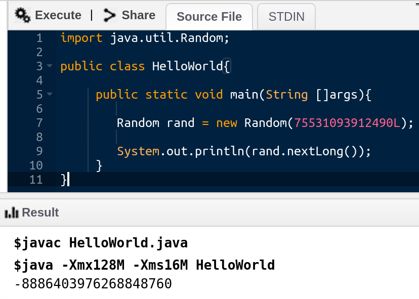
OWASP Benchmark generated value:
-8886403976268848760
Reminder: based on the source code of OWASP Benchmark, the Random() object gets initialized with the value returned by Java.lang.System.currentTimeMillis().
As such, using the extracted seed, it’s possible to calculate the local time of the server. Using this knowledge and by running our algorithm in the forwards direction, it’s possible to predict the value assigned to future cookies, thus facilitating a session hijack attack.
Final words
This post is an introductory text to Z3; a SAT solver from Microsoft Research. The post demonstrates basic usage of Z3, constraint generation and solution extraction. Additionaly, we demonstrate how Z3 can be used to symbolically execute a PRNG algorithm and extract hidden internal states using algorithm output. Finally, we demonstrate this ability using OWASP Benchamrk and show how the approach can be used as a weak PRNG detector.
While similar examples can be found around the web (including a book by Dennis Yurichev who inspired this post, see below), we couldn’t find a structured introductory text. It is our hope that this post provides a good intro for Z3, demonstrates its use for analyzing source code and sparks interest in the approach among security professionals.
Notes & Sources
Code repository with examples detailed in the text
Patched version of Z3 integrated with Jupyter notebokk
Book by Dennis Yurichev with many worked Z3 examples
Reverse engineering demo using Cutter and Z3
Background
Boolean satisfiability problems